Hidden Complexity of Time Series Data & Cleaning Guide

Time is arguably the most valuable dimension in any dataset. Whether you are tracking product usage, monitoring industrial sensors, or watching financial markets tick by tick, it is the temporal ordering that lets an organization reason about change rather than just state.
On the surface, a time series looks like nothing more than a column of values stamped with timestamps. In practice it is a far more fragile object. A single dropped sensor reading, a delayed batch load, a clock that drifts a few milliseconds, or a duplicated event can quietly corrupt the very structure that makes the data useful, namely the dependency between each observation and the ones before it.
That fragility is precisely why time-series analysis has become a discipline of its own. The hard part is getting a dataset that is consistent, correctly ordered, and faithful to what actually happened in the real world, and then reckoning with what that data still cannot tell you. This guide walks through both halves of that problem: the engineering work of producing trustworthy time-series data and the limits of relying on history alone.
What Makes Time-Series Data Unique?
A time-series dataset differs from a conventional tabular dataset in one decisive way: order is not optional; it is part of the meaning. In a standard table you can shuffle the rows and lose nothing. Shuffle a time series and you destroy it, because each value derives its significance from its position in the sequence and its relationship to neighboring values.
Consider retail analytics. A spike in transactions at 6 p.m. on a Friday might reflect a payday pattern or a flash promotion. Strip away the temporal order and that spike becomes indistinguishable from random noise instead of a signal tied to real behavior.
Key characteristics of time-series data
A few properties recur across almost every real series, and a competent analyst reasons about them explicitly:
Trend: A long-run direction in the level of the series, upward or downward, independent of short-term fluctuation.
Seasonality: Repeating patterns tied to a fixed period: hour of day, day of week, or month of year. Seasonality is regular and predictable in its period.
Cyclicity: Longer, irregular swings (business cycles, demand cycles) that are not anchored to a fixed calendar period and are easily confused with seasonality.
Autocorrelation: The defining trait: a value is statistically correlated with its own past. This is what makes forecasting possible and careless data handling so destructive.
Stationarity: Many classical methods assume that the statistical properties (mean, variance, autocorrelation structure) remain stable over time. Real-world series are frequently non-stationary, and recognizing that, then differencing or detrending appropriately is a prerequisite for sound modeling.
Why Time-Series Data Becomes Messy
In production systems, time-series data is almost never clean at the point of collection. Even mature pipelines emit imperfect records, and the root cause is usually systemic rather than human.
Where the issues come from
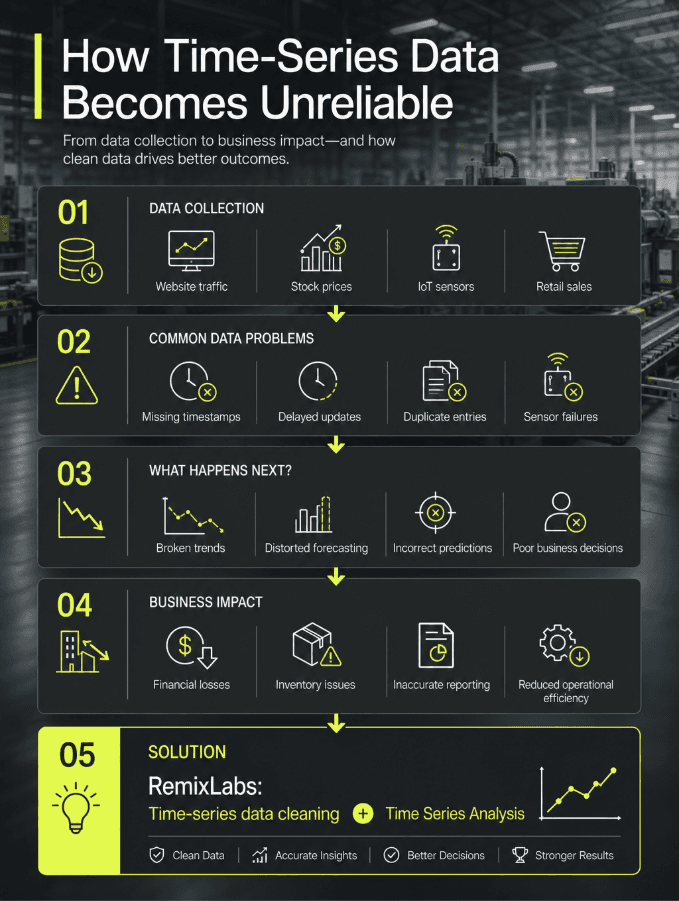
A device can hang for a few seconds, an API can throttle or time out, a network partition can interrupt the stream, or a downstream consumer can fall behind and drop messages. At the scale of an IoT fleet or a high-frequency trading feed, a few seconds of disruption produces visible, structured gaps rather than scattered noise.
There are also subtler problems. Different source systems log at different cadences, some on fixed intervals and some only on events, so aligning them onto a common timeline is non-trivial. Clocks drift, time zones are recorded inconsistently, and batch jobs land late, all of which create timestamps that look plausible but are wrong.
The Core Problem: Missing Time-Series Data
Few defects are as damaging as missing observations, because time-series work depends on continuity. In a static dataset you can drop a row and move on. Drop a row from a time series and you have broken the sequence, which distorts autocorrelation estimates, biases seasonal decomposition, and degrades any forecast built on top.
It also matters why the data is missing. Statisticians distinguish three mechanisms for missing data, and this distinction is not merely academic:
Missing Completely At Random (MCAR): The gap is unrelated to any value, observed or unobserved. The easiest case.
Missing At Random (MAR): Missingness depends on other observed variables but not the missing value itself.
Missing Not At Random (MNAR): Missingness depends on the missing value, for example, a sensor that saturates and drops out precisely during the extreme event you most need to capture. This is the dangerous case, because naive imputation will systematically understate exactly the behavior that matters.
Missingness also takes different shapes: isolated single-point gaps, long contiguous blocks from an outage, or sparse random dropout scattered through the series. Each type of missingness calls for a different remedy, and applying the wrong one quietly introduces bias into everything that follows.
Time-Series Data Cleaning: The First Critical Step
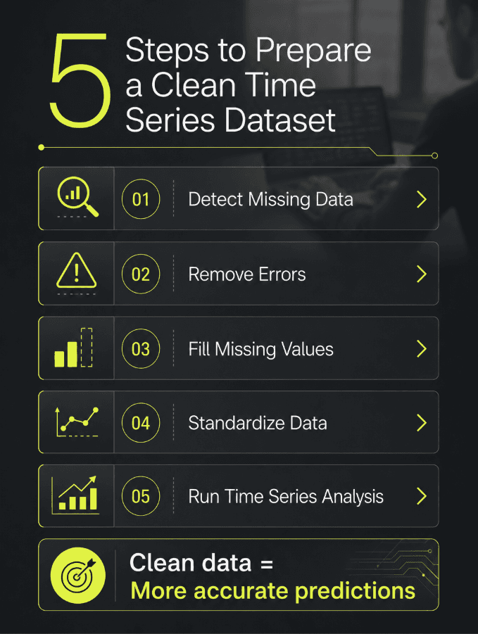
No modeling should begin before the series has been cleaned, because every downstream technique inherits the flaws of its input. Cleaning is what makes the dataset consistent, continuous, and true to reality.
Handling missing values and inconsistencies
Imputation is usually the first task, but it is a modeling decision, not a clerical one. The crucial constraint in a forecasting context is to avoid look-ahead bias: an imputation method must not use information from the future relative to the point being filled, or you contaminate the evaluation and overstate accuracy.
Beyond the gaps themselves, you also have to resolve duplicate timestamps, out-of-order events, irregular intervals, and format inconsistencies, all of which are easy to miss and quietly corrupt joins and aggregations.
Managing outliers and noise
Real series contain sudden spikes and drops that do not reflect genuine behavior, often from sensor faults or transient glitches. Robust detection, for example, rolling median with median-absolute-deviation thresholds or z-scores computed on seasonal residuals rather than raw values, separates noise from the signal.
The hard judgment is distinguishing a true outlier from a genuine event, a structural break, or a regime change. Aggressively "cleaning" anomalies away can erase the very signal a stakeholder needs to see. The goal is to correct artifacts without sanding off reality.
Standardization and alignment
Finally, the dataset has to be standardized: normalize all timestamps to a single canonical time zone (typically UTC, with offsets preserved), reconcile units of measurement, and resolve daylight-saving discontinuities.
When sources arrive at different cadences, resampling brings them onto a common grid, downsampling with an appropriate aggregation (sum, mean, or last) and upsampling with controlled interpolation. Without this alignment step, even clean data produces inconsistent results once series are combined.
Methods for Handling Missing Time-Series Data
There is no universally best imputation method; the right choice depends on the gap structure, the dynamics of the series, and how the result will be used.
Simple imputation approaches
Forward fill (last observation carried forward) and backward fill are cheap and intuitive, and they are reasonable for slow-moving, step-like signals such as a thermostat setpoint. The catch is that they flatten variance and can mask real movement, so they are a poor fit for volatile series.
Interpolation-based methods
Interpolation estimates missing points from their neighbors. Linear interpolation draws a straight line between known values and assumes local linearity, which is fine for short gaps. Spline interpolation produces a smoother curve that better tracks gradual change, at the risk of overshooting around sharp transitions. Both degrade as gaps widen.
Statistical and model-based approaches
More principled methods model the series itself. ARIMA and SARIMA capture autoregressive structure and seasonality, while state-space models with a Kalman filter or smoother go further, representing the series as a latent process and propagating uncertainty through the gaps, with native support for multivariate series. These approaches are more involved to specify and validate, but they respect the temporal dynamics that simpler fills ignore.
Machine learning methods
Increasingly, teams use ML to impute, framing the problem as predicting the missing value from lagged features and correlated series using gradient-boosted trees or temporal neural networks. Multivariate approaches exploit cross-series correlation, inferring one sensor from the behavior of related ones. The trade-offs are real: these models can overfit, demand careful feature engineering, and are especially prone to leakage if future information sneaks into the training window.
Real-World Impact of Poor Time-Series Quality
Low-quality time-series data still run in a model, but the cost surfaces downstream where decisions are made. In finance, distorted inputs produce mispriced risk and poor trade signals. Whether in finance or retail, data quality directly impacts business outcomes. Missing data can delay critical decisions, while corrupted data streams can generate false signals, or worse, hide genuine risks, operational issues, or revenue-impacting events.
The pattern is the same across every industry: if you cannot trust the data, you cannot trust the decisions based on it. Data quality is consistently among the strongest determinants of how well analytics and forecasting perform in production.
Building a Reliable Time-Series Dataset
A robust dataset is the product of a deliberate, repeatable workflow, not a one-off cleanup. A defensible pipeline typically includes:
Reliable collection that minimizes interruptions and records collection metadata.
Validation gates (data contracts) that reject or quarantine duplicates, schema drift, and missing timestamps at ingestion rather than discovering them weeks later.
Cleaning and imputation were chosen for the specific gap structure and applied without look-ahead bias.
Standardization and resampling onto a consistent schema, time zone, unit set, and interval.
Testing and visualization before modeling to confirm the series behaves as expected.
Lineage and governance ensure that every transformation is reproducible and that every downstream consumer knows what was done to the data and who is allowed to see it.
That last point is where many otherwise-solid pipelines fail to deliver, and it is where most of the business value is gained or lost.
The Limits of Historical Data: What Cleaning Cannot Fix
Here is the constraint that gets too little attention. Even an immaculate, well-governed time series has a ceiling on what it can teach you, because it only contains what actually happened. Cleaning repairs the record of the past; it cannot manufacture coverage of events that never occurred.
That gap matters most exactly where the stakes are highest. The rare regime, the extreme spike, the demand shock, the failure mode you have not yet lived through, these are sparse or absent in your history. A model trained only on observed data is effectively blind to them, which is why systems often perform well in normal conditions and fail precisely when conditions turn unusual. Waiting to collect more real data is slow, expensive, and, for genuinely rare events, may never happen at all. So the question shifts from "how do I clean what I have?" to "how do I responsibly extend what I have to cover the scenarios I need to prepare for?"
How Remix Labs Fits into the Time-Series Workflow
This is where a platform like Remix Labs plays its part, and it is worth being precise about which part. Remix is not a data-cleaning or imputation engine; the engineering work above still belongs to your pipeline. Remix sits one step further on it: it is a no-code platform for synthesizing new time-series datasets from your existing data, so you can model and test against scenarios your historical records do not contain.
In practice, that means a few things for time-series workflows:
It extends your data without new collection. Using the patterns already in your real series, Remix Labs creates extra time-series scenarios that are useful for stress-testing assumptions, adding to training data, and exploring conditions you have not yet seen.
It targets the rare and the extreme. The point is to model situations that are sparse or absent in history, such as unusual regimes and extreme events, rather than only the conditions you have already lived through.
It is built for analysts, not just engineers. A no-code, visual workflow lets analysts and developers build and run synthesis pipelines without standing up custom infrastructure or waiting on a data-engineering backlog.
It is repeatable. Because a synthesis run is configurable and reproducible, you can regenerate a dataset with the same settings, which keeps experiments and validation consistent over time.
For data teams, the payoff is the ability to prepare for scenarios their raw history never captured. The cleaning and modeling remain disciplines in their own right; Remix Labs addresses the separate problem of coverage, giving analysts more to work with than the past alone provides.
Conclusion
Strong time-series insight rests on two foundations, and most teams invest heavily in one while neglecting the other. The first is honest data engineering: recognizing that real series are noisy, non-stationary, and incomplete by default, and applying the right tool, interpolation, state-space modeling, or machine learning, to each specific failure mode without introducing bias or leakage. The second, easily overlooked, is coverage: accepting that even a clean history is a limited record of the past and finding responsible ways to test against the rare and extreme scenarios it does not contain.
As more industries push forecasting and automation onto time-based data, both foundations grow more consequential. Better data yields better models, and broader scenario coverage makes those models far more robust when conditions turn unusual.
Want to model the scenarios your historical data has never captured?