Why Raw Time-Series Data Breaks Down and How to Fix It Fast

Raw time-series data looks trustworthy on a chart. Underneath, though, it hides gaps, drift, and blind spots that quietly wreck models. We now generate more of this data than ever. IoT Analytics counted roughly 21.1 billion connected devices in 2025 and expects those devices to produce about 79.4 zettabytes of data, most of which are time-stamped. (https://iot-analytics.com/number-connected-iot-devices/)

Yet abundance is not the same as usefulness. Analysts often treat historical records as ground truth. Those records capture what already happened, not what could happen next. Sensors miss readings. Timestamps arrive out of order. Rare events are often overlooked.

Consequently, new models trained on this data inherit the flaws baked into it. Time-series data breaks in structural ways that standard fixes cannot reach. Understanding these cracks changes how you plan around them. First, let us see why the data itself misleads us.

The Illusion of Complete Historical Data

A system’s raw time-series data is a record of what was observed and little more. It will not put into perspective the scenarios that went unrecorded. Take a demand model: it is trained on the history of sales, but it has no experience with a supply shock yet to come. The model is left to prepare for yesterday rather than for tomorrow.

One could say this is where the problem lies. History is merely a sample and an incomplete one at that, with a bias toward the ordinary. Extreme events are conspicuous by their absence. Put simply, a model of raw history will underweight the moments of greatest consequence. Then there is the cost of poor data quality.

According to MIT Sloan Management Review, companies can be looking at a 15% to 25% hit to their annual revenue because of it. (https://www.integrate.io/blog/data-quality-improvement-stats-from-etl/)

The skew is technical in nature as well. Conventional approaches work on the premise of independent and identically distributed observations, an assumption that time-series data does not honor. There is excessive reliance on the previous days' value, and the mean and variance will change with the seasons or cycles.

Statisticians refer to such non-stationarity as a case of the rules changing in the real world. A historical window usually fails to show the breadth of behavior, and extrapolation compounds the issue. You end up with models making confident predictions from scant evidence, which can make a rare event seem impossible and lead to planning for the worst.

Where Raw Time-Series Data Breaks Down

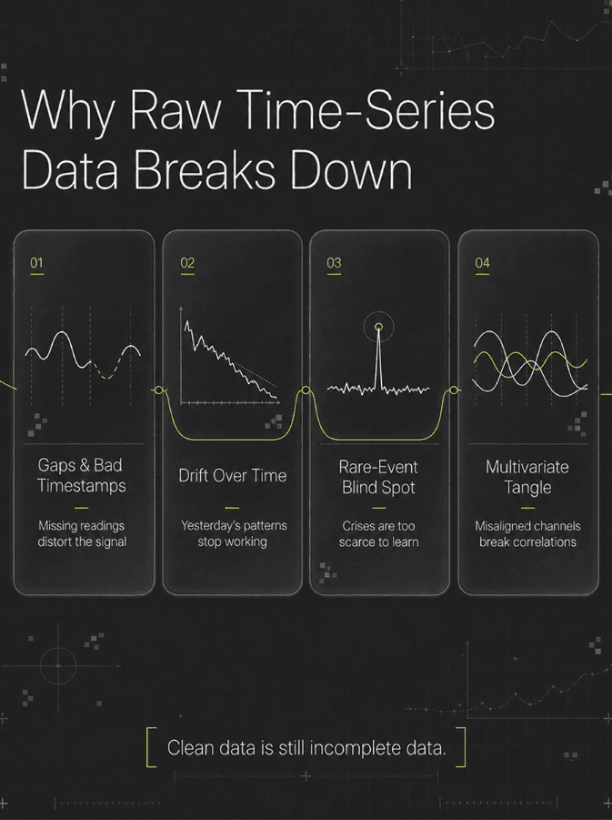
Raw time-series data fails in four recurring ways. Each one weakens the models built on top of it. Together, they explain why standard fixes fall short.

Gaps, Irregular Timestamps, and Missing Values

Real sensors drop readings. Networks stall. Devices reboot. Consequently, time-series files fill with gaps and uneven intervals. Many techniques for time series analysis assume a fixed sampling frequency. Irregular timestamps break that assumption immediately.

To address it, an analyst might resort to imputation, doing a forward-fill or some interpolation to plug the holes. But one has to remember that imputation is making up for values that were not actually recorded. It warps the kind of statistics that matter. Interpolation has a way of smoothing out volatility and making risk seem less than it is, while forward-fill will artificially flatten a trend by holding a value in place. Downstream metrics pick up on this quiet bias, and the numbers lose their connection to what is really happening.

Then there is the matter of how data goes missing. While some points are absent at random, others have a habit of vanishing under extreme conditions. The latter is the more perilous scenario, since the model lacks a signal when it is needed. Time itself can be a mess. You have clocks drifting from one device to the next, or duplicates appearing on a retry. Daylight Saving changes and time zones can disrupt the order.

By themselves these are small problems, but in combination they undermine the sequence the model is built on.

Distribution Shift Quietly Erodes Accuracy

The premise of time-series models is that tomorrow will be much like yesterday. The real world has other ideas. Markets are in flux, customer habits evolve, and equipment wears down. We refer to this gradual change as distribution shift or concept drift, and it is the reason a model put in place last year will not hold its accuracy today.

One should make a distinction between two types of change. There is covariate drift, where the inputs themselves move with time, and then there is concept drift, which alters the relationship between those inputs and the result. Both will undermine a model’s precision, but they call for different handling. The trouble is that looking at raw history does little to tell you what is at play, while the model continues to impose old patterns on new circumstances.

You see it in any review of production systems: as live data diverges from the training data, the model’s performance wanes. A monthly cycle for batch retraining may offer some relief, but drift is not bound by the calendar. Weeks can pass with diminished accuracy before the next retraining is due.

In the end, static historical data has its limitations; it is a record of one regime until the world moves on to another.

The Rare-Event Blind Spot

By their very nature, the most consequential events are uncommon. One must look at fraud spikes, outages, stockouts, or a sudden surge in demand to see that these occasions have significant business implications, even if they make up but a few rows in the historical record.

A model will therefore be presented with thousands of uneventful days and very few crises; it is only to be expected that it masters the former and struggles with the latter. Do not mistake this for an error in labeling. In the real world, you can only label what you have captured. The scarcity of extreme conditions makes this as much a matter of coverage as it is of mathematics.

Take a payments team contending with some novel form of fraud. If the tactic is almost absent from the logs of the past year, the model will struggle to identify it on any scale. Retailers run into the same difficulty when confronted with an unusual spike in demand.

Such tail events are where the major gains and losses are to be found, yet they remain obscured in the fringes of the distribution. In the end, you cannot properly stress-test a strategy based on data that lacks those events.

Why Multivariate Time Series Analysis Multiplies the Trouble

Single-series problems are already difficult, but multivariate time series analysis makes things even more demanding. In a real system one is tracking numerous signals in tandem: usage, prices, weather, sensor data, and so on.

The trouble is these channels do not always behave in concert. They are sampled at varying rates and have their own lagged, entangled dependencies. Consider a scenario that has to account for demand, price, and weather; a shift in price today might not show up in the demand figures for three days.

The model must ensure that those lags are consistent across all data. If the timestamps are at odds, it will infer a relationship that is not there, and even a minor misalignment can lead to substantial forecasting error.

Then there is the matter of missing data. A void in one channel will taint the relationships in another. Correlations the model depends on will quietly unravel if a series starts to drift. With different sensors going down on different days, the overlap of usable data between channels diminishes, leaving an effective dataset that is not as robust as it seems. Advanced methods struggle with panels that are incomplete or misaligned. All the above flaws compound the complexity, and any feature engineering done across the channels only serves to make the whole thing more fragile.

Cleaning Is Necessary, but Not Sufficient

Data cleaning clearly matters. Teams also pour enormous effort into it. In fact, industry surveys show a consistent pattern. Data professionals spend most of their time preparing data, not analyzing it. Anaconda's research adds detail here. Cleaning and organizing alone can consume over a quarter of the average data workday.

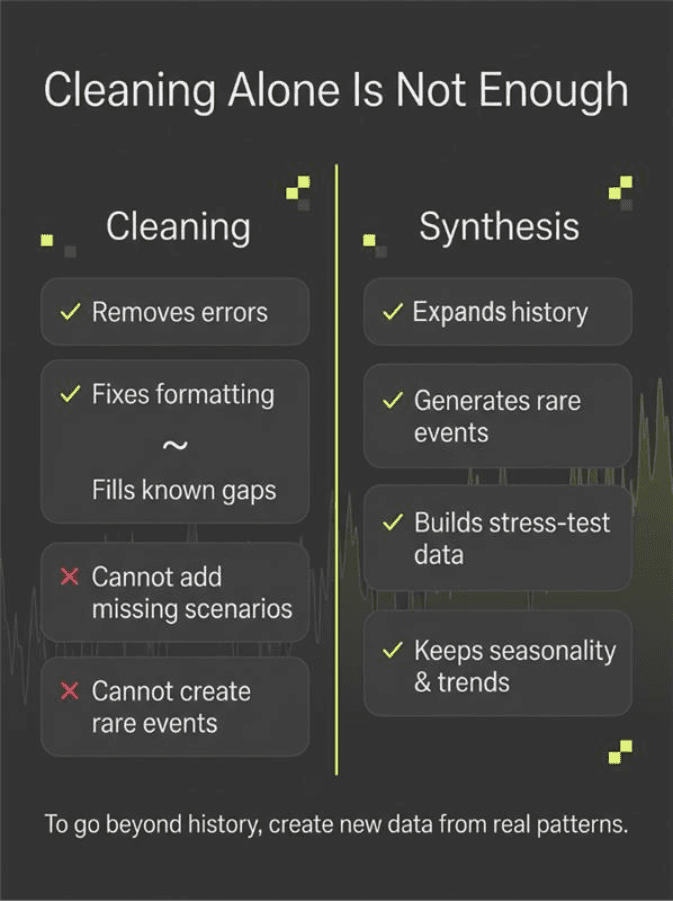
Yet cleaning only removes errors from what already exists. It cannot add the history of rare regimes. It also cannot manufacture the stress scenarios you need for testing. Therefore, cleaner data remains incomplete. The ceiling stays fixed by whatever the past happened to capture. To break that ceiling, teams need a different move. Specifically, they need a way to create new, realistic data from existing patterns.

From Cleaning to Data Synthesis

Synthesis flips the approach entirely. Instead of only repairing history, you extend it deliberately. A synthesis platform studies patterns in your existing series first. Then it generates new, realistic scenarios grounded in those patterns.

What a Synthesis-First Approach Delivers

This approach respects the structure of your real data. By way of augmentation, the process will vary seasonality, trends, and cross-channel links to come up with new and plausible scenarios. The idea is for your team to test ideas under conditions that ring true. One can even model for rare events by design.

On the training side, having more diverse examples helps a model learn to generalize, which in turn means it can be surer of itself with novel inputs. As a result, the forecasts are better able to stand up to changing circumstances.

Move Beyond Broken History with Remix Labs

Raw time-series data will present its usual problems: drift, misalignment, imbalance, and the odd gap. You can use a cleaning tool on its surface, but it will not create scenarios that your history has not already recorded. For that you need synthesis.

Remix Labs approaches it in another way entirely. We let you build new time-series datasets from what you have on hand. With our no-code visual pipeline doing the work, you simply upload the data and zero in on the relevant events to remix into something new. From there, built-in models like N-BEATS, NHiTS, LSTM, and GRU do their job.

The result is the ability to train more exacting models, put assumptions to the test, or even model rare occurrences that are not in your files. And there is no requirement for any fresh data collection.

If you are prepared to leave broken history behind, see what kind of results synthesis can yield over at remixlabs.ai.