Fixing Time-Series Data Without Losing Information

Time-series data underpins many of the systems organizations rely on every day, supporting retail analytics, financial operations, machine learning applications, and real-time operational monitoring. 

And for all its value, keeping that data in top shape is one of the most demanding tasks an organization faces. The cost and time devoted to nothing but data cleaning are at anywhere from 30% to 80% of a data warehouse's development, even as the market for quality solutions expands some 17% a year. (https://ieeexplore.ieee.org/stamp/stamp.jsp?arnumber=8943205) 

It is not as straightforward as patching up a missing value or ironing out an inconsistency. In a temporal dataset, a single careless edit propagates. Imputing a value reshapes every lag feature, rolling average, and autocorrelation estimate computed downstream from it. A hasty change can skew the behavioral patterns in the data, erase an event of consequence, or upset the temporal order that models depend on. 

Good time-series cleaning means preparing the dataset for analysis while keeping the important signals, trend, seasonality, and genuine anomalies intact. 

Why Time-Series Data Is Different 

Time series data is unlike ordinary tabular data: its temporal aspect puts a whole new spin on how you should handle the information. 

With ordinary tabular data, you are dealing with independent, identically distributed observations for the most part. You can take a transaction or customer profile and analyze it in isolation, and you can shuffle the rows without consequence, because nothing in one record depends on the row above it. 

However, time-series data behaves differently. 

Here the records form an ordered sequence where each observation is correlated with the ones around it, what statisticians call autocorrelation. The data carries trends, seasonality, and often non-stationary behavior, meaning its mean and variance drift over time.  

Because of this dependence, you cannot reorder rows, you cannot fill gaps with a column average, and you have to guard constantly against lookahead bias, where information from the future leaks backward into a record it should never have touched. The order in which the data is presented is as important as the data itself. 

The Hidden Cost of Poor Data Quality 

Poor-quality time-series data creates problems that extend beyond inaccurate reporting. 

Organizations frequently encounter: 

• Missing timestamps 

• Data gaps 

• Duplicate records 

• Misaligned sources 

• Inconsistent sampling frequencies 

• Fragmented event histories 

You will find that as these problems build up, they corrupt the whole data stack. Irregular timestamps break the lag and window features that ML models depend on; misaligned sources introduce silent join errors; and inconsistent sampling frequencies force resampling that can smear or alias real signals. The damage compounds as it moves from raw tables into feature stores, then into analytics, forecasting, anomaly detection, and operational monitoring. 

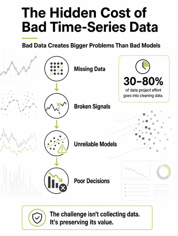
Gartner puts the average cost of substandard data at $12.9 million a year for an organization, all in the name of poor decisions and inefficiency. (https://www.gartner.com/en/data-analytics/topics/data-quality)  

With time-series systems, you can face even steeper costs, since any missing or skewed event can dictate how the system behaves down the line. Then there is the matter of resolving the issue; it is one thing to spot a data quality problem, quite another to put it right without losing the important signals in the process.

Understanding Missing Time-Series Data  

Missing data is one of the most common challenges in time-series environments. Unlike traditional datasets, missing observations often occur during important operational events. 

Common causes include: 

• Sensor outages 

• Pipeline failures 

• System downtime 

• Delayed ingestion 

• Communication interruptions 

It helps to know “how” the data went missing. Gaps that are missing completely at random (MCAR) are forgiving; missing gaps not at random (MNAR), where the outage and the event causing it are linked, are the dangerous ones, because the very moments you most need are the ones that disappear. The shape of the gap matters too: scattered point gaps respond well to simple methods, but long block gaps from an extended outage defeat most of them. 

Teams reach for a wide spectrum of fixes, from forward-fill and linear or spline interpolation through state-space methods like Kalman smoothing up to deep-learning imputers such as BRITS and SAITS.  

The researchers put it down to the fact that when you have real-world problems like an extended outage, even the most advanced models can flounder and end up introducing statistical bias into your data.  

This illustrates a key lesson: it is more valuable to keep system behavior realistic than to reach for the most complicated algorithm you can find. 

Validating That a Fix Preserved the Signal 

If the whole point is to clean data without losing information, then you need a way to prove you didn't lose any. Too many teams apply an imputation, eyeball the chart, and move on, which is precisely how silent bias enters a pipeline. 

The standard technique is masked, or holdout. Validation: Take a stretch of known-good data, artificially blank out points in the same pattern as your real gaps, run the imputation, and score the reconstruction against the values you hid. Pointwise error metrics, MAE, RMSE, and mean relative error give you the first read. 

But low pointwise error is not enough, and the next step is where most validation stops short. A fill can score well on RMSE while quietly flattening the data, because interpolation and mean-filling shrink variance and inflate autocorrelation.  

So, you check structure directly: compare the AutoCorrelation Function (ACF) and the power spectral density before and after and test whether the overall distribution has shifted using a Kolmogorov–Smirnov test or Wasserstein distance. 

The final and most honest test is downstream. Backtest your forecasting or anomaly-detection model on a held-out period and confirm that its performance holds on the repaired data. If the fix improved your error metrics but hurt the model, it was wrong. 

Best Practices for Fixing Time-Series Data 

Organizations looking to improve time-series data quality should focus on five core principles: 

1. Preserve Raw Data: Always maintain an untouched, immutable source dataset for validation, lineage, and auditing. 

2. Understand System Behavior: Cleaning decisions should reflect operational realities and the data's generating process, not generic assumptions. 

3. Flag Before Deleting: Where possible, mark questionable observations rather than removing them, so anomalies remain recoverable. 

4. Monitor Data Quality Continuously: Watch for distribution drift and schema changes; quality is an ongoing process, not a one-time project. 

Final Thoughts 

You can't put time-series data in order by simply plugging in missing values and removing the oddities. Time-series systems are a record of how things change over time, so any choice you make in the cleaning process can change what the data is telling you. Some organizations are so intent on churning out pristine datasets that they end up throwing out the very signals, the anomalies, and behavioral patterns needed for effective machine learning or operational insight. 

The teams that get the most from their data treat clean historical records as a starting point, not the finish line. Once the data is sound, the more valuable question is whether it covers the full range of conditions a system actually faces, including the rare events and edge cases history simply hasn't recorded yet. 

For teams ready to move past cleaning and toward getting more out of what they already have, that is where Remix Labs comes in, turning historical records into broader, more representative time-series datasets that strengthen analytics, machine learning, and operational resilience.